Trading strategy simulation with Python

Whether you’re a new or an existing investor, you probably have heard of the term dollar-cost averaging, which refers to an investment strategy that alleviates the emotional stress and investment risk by dividing up the total amount to be invested across periodic intervals.

There are studies by institutions such as Vanguard back in 2012 that compared the historical performance between dollar-cost averaging (DCA) and lump-sum investment (LSI). It concluded that on average, an LSI approached outperformed DCA approximately two-thirds of the time, even after adjusting for higher volatility of a stock/bond portfolio. Investing in a lump sum gives investor exposure to the markets earlier, which is especially beneficial if the markets are upward trending in the long term.

However, psychology plays a crucial part in investing. More often than not, an investment decision is made out of fear or greed. There are numerous stories out there about people making or losing money because of FOMO or YOLO.

I really enjoyed the book The Psychology of Money by Morgan Housel. In the book he pointed out that

The trick when dealing with failure is arranging your financial life in a way that a bad investment here and a missed financial goal there won’t wipe you out so you can keep playing till the odds fall in your favor.

So in this article, I would like to continue exploring the idea of dollar-cost averaging, by tweaking the trading frequencies to understand how risk and return of assets may vary accordingly.

Assumptions and Methodology#

I’m typically interested in comparing weekly (5-day) vs monthly (20-day) investment interval. The dataset is pulled via the Python package yahoofinancials. Backtesting is done by randomly sampling historical prices over a 5-year period since 2016 to construct portfolios.

Before getting into simulation, below are some of the assumptions embedded in the model:

Same starting time and same total dollar amount to be invested over the studied period
Assuming partial stock can be bought and traded at the close price (reason for using closed price will be explained below. This can also be adjusted for any other price)
Assuming zero brokerage fee
Weekly trading picks a random price point (rather than every 5th day) to invest, for every 5 pricing points bundled together chronologically. Same applies to the monthly approach
At each trade, the amount invested is fixed and depends on the trading frequency, i.e. higher amount to be invested for monthly vs weekly
% return is calculated by comparing total amount invested to date v.s. the current portfolio value

Exploratory Data Analysis on Historical Prices#

An important step to take before any modelling or simulation is to actually look at the data we are analysing. Furthermore, to simplify the simulation process, I will only consider trading the price at either open or close.

If you are on Twitter, you might have come across this tweet:

I was going to write a book about trading but decided it could be boiled down into one Tweet:

Buy the Close - Sell the Open
— . (@StockCats_2009) February 5, 2021

To test the statement above, I pick QQQ, which includes the top 100 companies listed on Nasdaq, as an example. Here I compare the differences between open and close on the same day (left), as well as the price difference distribution between close and the next open (right).

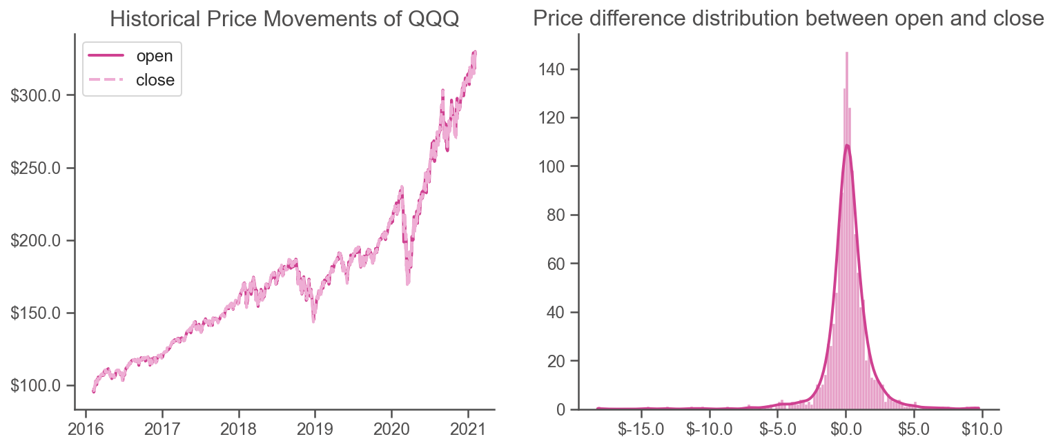
Interestingly, the price difference distribution resembles a normal distribution in real life for QQQ, which gives me confidence to use the test below for hypothesis testing:

Null: the difference between close and next open is 0
Alternative: the difference between close and the next open is > 0

# add difference between next open price and close as a new column
historical_price["diff"] = historical_price["open"].shift(-1) - historical_price["close"]

# hypothesis test on if the difference between historical open and close was > 0
scipy.stats.ttest_1samp(historical_price["diff"], 0, alternative='greater')

The test result returns a p value of less than 5%, suggesting it is statistically significant on average that the next day open is greater than the previous close for the selected ticker.

Simulating Dollar-cost Averaging#

In this section, I will go through the methodology used in simulating different trading frequencies of dollar cost averaging, and compare the risk and return for weekly (5-day) vs monthly (20-day).

Rather than investing every nth day, the algorithm randomly selects an available date and price within specified trading interval to mimic an individual investing a fixed amount consistently over the studied period.

Based on the pricing points randomly picked, the algorithm then computes the number_of_units at each trade, prices of the asset, total_dollar_amount_invested to date as well as the % return.

You can also choose how many times the simulation needs to be run to get an expected portfolio return and construct confidence intervals.

Below is a simulated return on investing a total of $50, 000 on QQQ from 2016 to date, where value_w represents investing on a 5-day interval and value_m is the 20-day interval.

According to the figure, it looks like the monthly one has a different total value of return v.s. the weekly one. Once again, hypothesis testing is applied to see if the two simulated values are different by constructing 10,000 portfolios respectively. The two-sided test returns a p value of 0, which suggests different yields by these two trading frequencies.

Risk usually goes hand in hand with return. Here, risk analysis is simplified by looking at the variances in returns. Levene test is performed for equal variances. The p value returned is 0.976, indicating not a significant difference in variances of returns by trading either weekly or monthly.

# perform Levene test for equal variances
scipy.stats.levene(result_w["return"], result_m["return"])

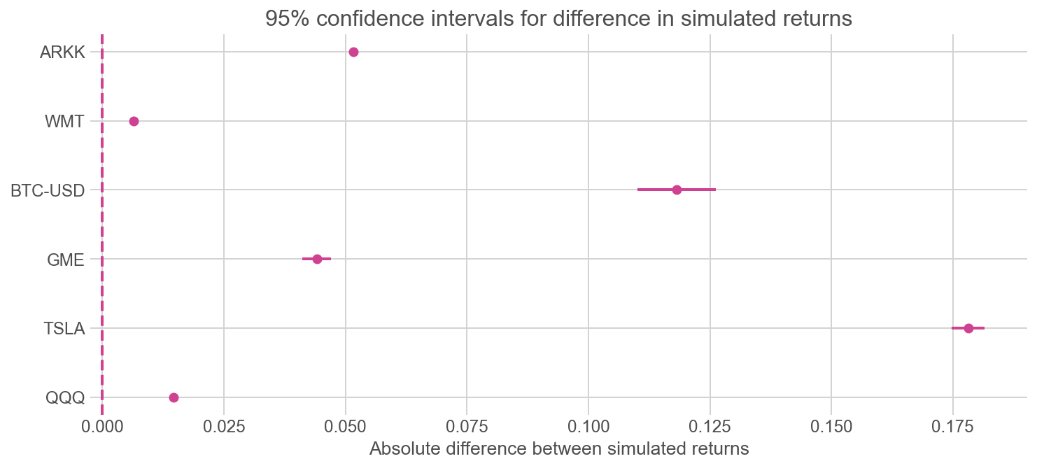
We can extent the analysis further by looking at multiple assets and their simulated performances over the past five years. In this example, I chose QQQ, TSLA, GME, BTC-USD, WMT and ARKK.

For each of the ticker above, I run simulations with the two trading strategies to construct 10,000 portfolios each, and compute 95% confidence interval for the absolute difference in percentage of returns.

We can see that all the monthly strategies outperform weekly ones under simulation. The returns are typically higher for volatile assets such as Bitcoin and TSLA, with wider confidence interval. In contrast, blue-chip stocks like WMT and index ETFs such as QQQ have an extremely narrow confidence interval, but also relatively lower incremental positive returns.

Furthermore, taking volatility into accounts, there is not significant difference in the variance of returns in both weekly and monthly trading strategies based on simulated results.

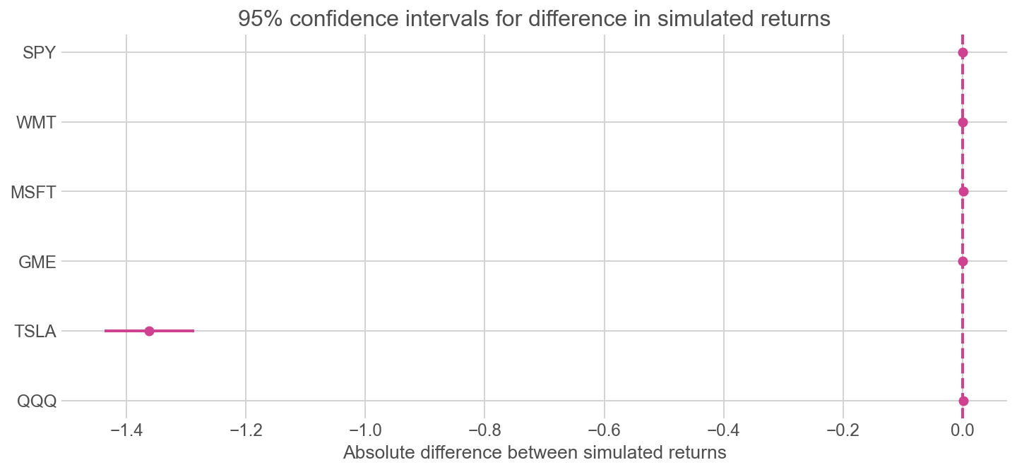
2020 was seemingly a phenomenal year for equities. To provide a full picture, it is also worth comparing the performance of two trading strategies under a rather turbulent macro environment.

Below are the difference in performances of QQQ, TSLA, GME, MSFT, WMT, SPY from 2007 to 2012, during which the market was hit by the Global Financial Crisis and subsequently the European sovereign debt crisis.

Out of the selected tickers, TSLA is the only asset where monthly trading severely underperforms the weekly one, and variances of returns are different. The rest yield no difference in terms of return and also display similar risk profile.

Conclusion#

If the market is trending upward in the long term, the simulated results indicate that a monthly trading interval with higher amount invested outperforms the weekly one. It generates statistically significant better returns and has similar volatility(a.k.a. risk) in our simulated portfolios.

In a market where assets are appreciating in value, it is logical to allocate more money earlier than later to get the exposure. However, the outcome could vary depending on which asset you invest on, and the expected return is more volatile for risky assets.

If interested, you can find all the work above in this repository.

Disclaimer

This post is provided for informational purposes only, and should not be relied upon as legal, businesses, investment or tax advice. References to any securities or digital assets are for illustrative purposes only, and do not constitute an investment recommendation or offer to provide investment advisory services.